Online Dating: Quarantine Edition

You did it. You really did it.

You finally succumbed to quarantine fever and used your credit card to pay the membership fee for Match.com.

Of course, you’re skeptical about the whole “online dating” thing, but you’re optimistic and hopeful—and probably a little excited by the idea that true love might be (literally) just a mouse click away. Really, though, you’re just hoping the opportunity cost of spending $23.99/month will be worth it when you [sigh] finally meet that twenty-something, super-rich [insert famous celebrity here] look-alike who is (1) still single (no chance), (2) also a member of Match.com (never happen), and (3) of the opinion you’re more attractive than anyone else they could ever meet (highly unlikely). But you still play the lottery, so you believe anything is possible. (It’s an unfortunate consequence of our sociosexual evolution that callipygian gifts require payment in kind. I think Aristotle said that.)

Anyway, what now? Endless scrolling? Interminable thanks-but-no-thanks messages followed by hasty profile blocking? Wasted Friday and Saturday nights trying to get not-quite [said famous celebrity] 2.0 with the slightly unattractive aquiline profile to pay more attention to you than the comments on their Instagram selfies? There’s a better way. Say “no” to bad lighting and undercooked meat, and say “yes” to ~~the dress~~ the mathematics of probability optimization.

Proba…what?

Right.

What if I told you we can use the power and beauty of mathematics to give you the best chance of finding the ~~lust~~ love of your life? It’s true. Let’s say you’re willing to look at a total of t profile pictures sent to you by Match.com’s ostensibly preternatural algorithms. By rejecting the first r pictures, you will maximize the probability of finding your “ideal match.” (Call this person x.) I know: you don’t believe it, but it really is that simple. So, what’s the value of r for a given t? Technically, the answer is $te^{-1},$ but we’ll get to that.

First, some ground rules:

Once you pass on a profile pic, you can’t go back. That person is gone forever. [insert crying emoji]
Once you choose the value for r, you must reject every person from the first to the rth.
You must choose the first profile (x > rth) that’s better than all the others you’ve seen.
You must choose the last profile you see if you haven’t chosen anyone to that point.
Once you choose someone, they are guaranteed to accept.

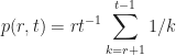
So, what do we know? Well, unfortunately, if your ideal match happens to show up within the first r profiles, you’re sunk. Because of rules 1 and 2, the probability of picking x—assuming x happens to arrive within the first r profiles—is, well, zero. To optimize your chances of picking x, we need to pick the optimized value for r. And to do that, we need to calculate the probability of x‘s location as Match.com sends profile pics to your inbox.

Okay, you can’t pick anyone within the first r profiles, but what if the (r+1)st profile is your dream date x? You’ll pick that person for sure, right? So, the probability is 1. But the probability of the (r+1)st profile being your dream date is (gulp) the worst it could be: 1/t (assuming a uniform distribution of profile pics). We take the product of these values; that is, “the probability you’d choose the (r+1)st profile assuming that person is better than the other r profiles” multiplied by “the probability this person happens to be located at the (r+1)st position in Match.com’s algorithm.” That happens to be [drum roll, please] (1)(1/t) = 1/t. For large t, that’s not so good. It gets better, though.

What if x is the (r+2)nd profile in your inbox? Well, you wouldn’t pick x in this scenario unless the (r+1)st profile wasn’t better than all the previous r profiles; in other words, the highest-rated profile to that point (i.e., the moment you received the (r+1)st profile) was one of the previous r profiles (otherwise, you would’ve picked the (r+1)st profile). The probability that the highest-rated profile of the first (r+1) profiles arrived within the first r profiles you rejected is very high, r/(r+1), and the probability that x happens to arrive in the (r+2)nd position remains 1/t. This is really the tricky part of the whole concept, so do yourself a favor and make sure you get it straight.

So, the total probability of the (r+2)nd profile being your dream date is the product of the two probability values we already calculated, that is, $t^{-1}\cdot r(r+1)^{-1}=r[t(r+1)]^{-1}.$ Probabilities for the (r+3)rd, (r+4)th, . . . , (t-2)th, (t-1)th, and tth profiles are calculated similarly, and we simply sum the individual probability values:

$p(r,t)=t^{-1}+r[t(r+1)]^{-1}+r[t(r+2)]^{-1}+\cdots+r[t(t-1)]^{-1}$ ,

and after factoring out r/t, this simplifies to

$\displaystyle p(r,t)=rt^{-1} \sum_{k=r+1}^{t-1} 1/k$ ,

which is simply an r-mulitple of the average of the individual probabilities the jth candidate will be x with $j = r+1,r+2,\cdots,t-1.$ Now, if we’re going to give you the best chance of finding your ideal x, we need to optimize the value for r. In other words, giving you the best odds requires knowing how many r profiles you must be committed to rejecting given an arbitrary number of profiles t. This means we need to optimize $p(r,t)$ and that requires $p(r,t)>p(r-1,t),p(r+1,t)$ for arbitrary t. The trick is to substitute r-1 and r+1 into the above equation and solve the inequalities.

Taking the first case, we have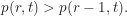 $p(r,t)>p(r-1,t).$ After substitution, we have

$\displaystyle rt^{-1}\Big[r^{-1}+(r+1)^{-1}+\cdots + (t-1)^{-1}\Big]>$
$\displaystyle (r-1)t^{-1}\Big[(r-1)^{-1}+r^{-1}+(r+1)^{-1}\cdots+(t-1)^{-1}\Big]$ .

Multiplying by t and distributing r-1 into the first term on the RHS gives us (1)

$\displaystyle r\Big[r^{-1}+(r+1)^{-1}+\cdots + (t-1)^{-1}\Big]>$
$\displaystyle 1+(r-1)\Big[r^{-1}+(r+1)^{-1}+\cdots + (t-1)^{-1}\Big]$ .

Notice the bracketed expressions in both the LHS/RHS are equal! Now, we only have to deal with coefficients. Let’s do that. Subtracting the LHS from the RHS leaves us with

$\displaystyle 0>1-\Big[r^{-1}+(r+1)^{-1}+\cdots + (t-1)^{-1}\Big]$ ,

which, after rearranging, becomes

$\displaystyle r^{-1}+(r+1)^{-1}+\cdots + (t-1)^{-1}>1$ .

If we substitute r+1 into inequality (1) above and follow a similar calculation, we arrive at the other inequality we need:

$\displaystyle (r+1)^{-1}+(r+2)^{-1}+\cdots+(t-1)^{-1}<1$ ,

yielding the final result (2):

$\displaystyle \sum_{k=r+1}^{t-1} 1/k < 1 < \sum_{k=r}^{t-1} 1/k$ .

At this point, we can find the optimized value for r given an arbitrary t. Just make sure the above inequality still holds. For example, imagine Match.com sends you, say, seven profile pics. Then, we have 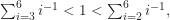$\sum_{i=3}^{6} i^{-1} <1<\sum_{i=2}^{6} i^{-1},$ and r = 2 because 19/20 < 1 < 29/20 holds.

What does this mean? Well, given a total pool of seven profiles from which to choose (adhering to the aforementioned restrictions), you would automatically reject the first two profiles—no matter who they were—and then choose the very next profile that was better than the first two you rejected. Note: To calculate r, we use the smallest number of terms (based on the value of t we chose) to satisfy both sides of the inequality in (2).

Here are some calculations using the above machinery:

$t = 3,\,\, r = 1,\,\, p\approx 0.5$
$t= 8,\,\, r = 3,\,\, p\approx 0.41$
$t=10,\,\, r = 3,\,\, p\approx 0.40$
$t = 30,\,\, r = 11,\,\, p\approx 0.38$
$t= 50,\,\, r = 18,\,\, p\approx 0.374$
$t= 100,\,\, r = 37,\,\, p\approx 0.37$
$t= 1000,\,\, r = 369,\,\, p\approx 0.368$

So, if you decide to consider a pool of 50 Match.com profiles, you’d automatically reject the first 18 and choose the first profile better than any of those 18 you rejected. That will give you a 37.43% chance of finding your ideal love match. Sure, you have about a 63% chance of missing x using this strategy, but any other strategy you choose will decrease your odds (assuming you follow the rules).[1]

One thing we can’t fail to notice is that as t gets larger, our p-value begins to settle around 37%.[2] That’s not a coincidence. In fact, the above inequalities relate to (a bounded subset of) the harmonic series: $\sum_{i=1}^{\infty} 1/i.$ All the denominators in our rational terms are conterminous positive integers that begin from r or r+1 and terminate at t-1. (Check this.) So, our work thus far can be recast as a function $f:\mathbb{Z}^+\rightarrow\mathbb{Q}$ of our two variables $r,t$ —defined by the RHS inequality—based on how we interpret the (upper and lower) Riemann sums of the integral, the meshes of which are simply the areas given by our chosen subseries of $H_n.$

Taking the RHS, we have

$\displaystyle \int_{r}^{t}\!\!x^{-1}=\Big[\ln x\,\Big]_{r}^{t}=\,\ln\Big(\frac{t}{r}\Big)\,<\,\sum_{i=r}^{t-1} 1/i$ ,

and the LHS is

$\displaystyle \sum_{i=r+1}^{t-1} 1/i < \int_{r}^{t-1}\!\!x^{-1}=\Big[\ln x\Big]_{r}^{t-1}=\ln\Big(\frac{t-1}{r}\Big)$ .

Putting it all together, we have

$\displaystyle \sum_{i=r+1}^{t-1} 1/i < \ln\Big(\frac{t-1}{r}\Big)<1<\ln\Big(\frac{t}{r}\Big)<\sum_{i=r}^{t-1} 1/i$ .

As t and r grow larger, however, we find that

$\ln\,(t-1)r^{-1}\approx\ln\,tr^{-1}\approx 1$ ,

and the last inequality above suggests we’re “squeezing” the value of 1 from both sides, yielding the final calculation:

$\displaystyle \ln tr^{-1}\approx 1\,\,\longrightarrow\,\,tr^{-1}\approx e\,\,\longrightarrow\,\,r\approx te^{-1}$ ,

as claimed.

What’s great about this is that your chances don’t decrease the larger t is. Whether you’re willing to look through 15 profiles or 15,000, your optimized probability remains the same—about 37%. Also, the variable t doesn’t have to deal with profiles; it could involve, say, time. If you’ve allocated five months to find the best venue for your wedding, you’ll reject everything you see until (about) day 56 (= 150/e), at which point you’ll choose the first venue that’s better than every venue you’ve seen so far. Of course, venues aren’t like jilted dates: you can always circle back and choose a venue you’ve rejected, but the math works the same way given the assumptions.

So, there it is. You have nearly 2/5 probability of finding your ideal date using the above approach. That’s pretty good, actually. It’s not as good the probability the sun will rise tomorrow, but it’s a lot better than getting even a short-term run in the stock market.

Math even cares about your love life.

Footnotes:

[1] Some strategies alter your chances by modifying our restrictions (e.g., selecting merely one of the best candidates, allowing proposal rejections, having full information about the candidates, incurring costs to passing, etc.). (As an example, one prominent design suggests stopping at $e^{-1/2},$ as opposed to 1/e.) Many people consider the classic optimization problem to be unrealistic for these reasons. Of course, this is silliness: The math just gives you the best chance of finding x; it doesn’t say anything about the chances of being accepted by x or living happily ever after with x or whether you would consider less optimal candidates y and z to be desirable replacements. That’s up to you, but $p=1/2e$ seems worth the rejection risk!

[2] This is why “no-information” optimal stopping is often referred to as “the 37% rule,” an algorithm originating in 1949 as Flood’s “fiancee problem“—recontextualized as “the secretary problem“—and later popularized by Martin Gardiner in the February 1960 issue of Scientific American.

References:

[1] B. Christian and T. Griffiths, Algorithms to Live By: The Computer Science of Human Decisions, New York: Henry Holt and Company, 2016.

[2] J. Billingham, Kissing the frog: A Mathematician’s Guide to Mating, Plus Magazine, 9 (2008) 1-3.

Written by u220e

2020-04-11 at 1:38 pm

Posted in MATHEMATICS, POP CULTURE, PSYCHOLOGY

Tagged with 37% rule, Martin Gardiner, Match.com, online dating, optimal stopping, optimization, secretary problem

The Critical Strip